Analyzing Solutions#
While every mode matching that achieves perfect overlap should be equivalent in theory, in practice some solutions are much easier to implement and align than others. If a lot of degrees of freedom are offered to the solver, there may be many possible solutions, and it can hard to sift through them all to find the best one. To help with this, Beam Corset calculates a variety of metrics and two kinds of analysis plots to help you find the most practical solution.
[1]:
import numpy as np
import matplotlib.pyplot as plt
from IPython.display import display
from corset import Beam, ThinLens, ShiftingRange, mode_match
[2]:
# setup beam with some uncertainty for later analysis
initial_beam = Beam.from_gauss(0, waist=500e-6, wavelength=1064e-9, cov=np.diag([1e-2, 10e-6])**2)
desired_beam = Beam.from_gauss(focus=1.0, waist=100e-6, wavelength=initial_beam.wavelength)
lenses = [ThinLens(f, 10e-3, 10e-3) for f in [100e-3, 150e-3, 200e-3]]
ranges = [ShiftingRange(left=0.0, right=0.8)]
solutions = mode_match(initial_beam, desired_beam, ranges, lenses, max_elements=3)
print(f"Found {len(solutions)} solutions.")
Found 16 solutions.
We give the solver three different kinds of lenses to work with and allow up to three elements per mode matching to get a larger number of possible solutions to analyze.
Quantitative Analysis#
To analyze a solution quantitatively, we can look at its analysis attribute which is a lazily computed ModeMatchingAnalysis instance. The analysis object computes a variety of metrics like sensitives of the individual degrees of freedom and how they affect the final beam’s waist position and radius.
For example, one very good predictor of how easy a solution is to implement are the couplings between the different degrees of freedom. It essentially describes how easily we can optimize the mode matching by only moving one element at a time without having to move another element with it to keep the overlap high. A coupling close to $1$ or $-1$ means that we will see a significant drop in overlap if we don’t move these two elements together with a precise ratio, a coupling close to $0$ means that the two elements can mostly be adjusted independently of each other.
[3]:
print(solutions[0].analysis.sensitivities) # sensitivity matrix
print(solutions[0].analysis.couplings) # coupling matrix
print(solutions[0].analysis.grad_focus) # gradient of focus positions w.r.t. degrees of freedom
# ...
[[1090.830957   -709.42504392]
 [-709.42504392  481.2550677 ]]
[[ 1.         -0.97912949]
 [-0.97912949  1.        ]]
[ 2.59346633 -1.55990254]
We can get a quick summary of all these quantities and some additional information by calling its summary() method.
[4]:
solutions[0].analysis.summary() # all analyses and some more information in a dictionary
[4]:
{'overlap': np.float64(0.9999999992340538),
 'num_elements': 2,
 'elements': [ThinLens(focal_length=0.1, left_margin=0.01, right_margin=0.01, name=None),
  ThinLens(focal_length=0.1, left_margin=0.01, right_margin=0.01, name=None)],
 'positions': array([0.47235006, 0.73730081]),
 'min_sensitivity_axis': 1,
 'min_sensitivity': 4.812550676983611,
 'max_sensitivity_axis': 0,
 'max_sensitivity': 10.908309569986647,
 'min_cross_sens_pair': (0, 1),
 'min_cross_sens': 7.094250439163218,
 'min_cross_sens_direction': array([0.55011895, 0.8350863 ]),
 'min_coupling_pair': (0, 1),
 'min_coupling': 0.9791294890281759,
 'sensitivities': array([[10.90830957, -7.09425044],
        [-7.09425044,  4.81255068]]),
 'couplings': array([[ 1.        , -0.97912949],
        [-0.97912949,  1.        ]]),
 'const_space': [],
 'grad_focus': array([ 2.59346633, -1.55990254]),
 'grad_waist': array([ 0.0015902 , -0.00162705]),
 'sensitivity_unit': <SensitivityUnit.PERCENT_PER_CM2: Unit(ascii='%/cm^2', tex='\\%/\\mathrm{cm}^2', factor=0.01)>,
 'solution': ModeMatchingSolution(candidate=ModeMatchingCandidate(problem=ModeMatchingProblem(setup=OpticalSetup(initial_beam=Beam(beam_parameter=0.7381561686066243j, z_offset=0, wavelength=1.064e-06, gauss_cov=array([[1.e-04, 0.e+00],
        [0.e+00, 1.e-10]])), elements=[]), desired_beam=Beam(beam_parameter=0.029526246744264968j, z_offset=1.0, wavelength=1.064e-06, gauss_cov=None), ranges=[ShiftingRange(left=0.0, right=0.8, min_elements=0, max_elements=inf, selection=[])], selection=[ThinLens(focal_length=0.1, left_margin=0.01, right_margin=0.01, name=None), ThinLens(focal_length=0.15, left_margin=0.01, right_margin=0.01, name=None), ThinLens(focal_length=0.2, left_margin=0.01, right_margin=0.01, name=None)], min_elements=1, max_elements=3, constraints=[]), populations=[(ThinLens(focal_length=0.1, left_margin=0.01, right_margin=0.01, name=None), ThinLens(focal_length=0.1, left_margin=0.01, right_margin=0.01, name=None))]), positions=array([0.47235006, 0.73730081]))}
The sensitivity matrix is one of the most important metrics, that many other quantities are derived from. It is proportional to the Hessian of the mode overlap with respect to the degrees of freedom such that the positive loss in overlap around the optimum is approximately given by:
where \(\mathbf{S}\) is the sensitivity matrix and \(\Delta \mathbf{x} = [\Delta x_0, \Delta x_1, \ldots]^T\) is the vector of displacements in the degrees of freedom.
By default, the sensitivity is specified in units of \(\%/\text{cm}^2\) where typical values are around unity. This makes it very easy to estimate how much overlap is lost for a given displacement. For example if the sensitivity is \(1.5\,\%/\text{cm}^2\) and we displace the element by \(1\text{ cm}\), we can square it to get a loss of approximately \(1.5\%\) in overlap. If we displace it by \(2\text{ cm}\) the loss will be about \(6\%\).
The coupling matrix \(\mathbf{R}\) is the sensitivity matrix normalized by its diagonal elements in the same way, that the correlation matrix is derived from the covariance matrix:
You can find a list of all available metrics, their meanings, and how they are calculated in the ModeMatchingAnalysis class documentation.
Instead of calling the summary method on each solution individually, we can also simply display the SolutionList returned by the solver, which shows a table of all summaries at once.
[5]:
solutions
[5]:
| overlap | num_elements | elements | positions | min_sensitivity_axis | min_sensitivity | max_sensitivity_axis | max_sensitivity | min_cross_sens_pair | min_cross_sens | min_cross_sens_direction | min_coupling_pair | min_coupling | sensitivities | couplings | const_space | grad_focus | grad_waist | sensitivity_unit | solution | |
|---|---|---|---|---|---|---|---|---|---|---|---|---|---|---|---|---|---|---|---|---|
| 0 | 1.000000 | 2 | [f=100mm, f=100mm] | [0.47235006080138076, 0.7373008080807102] | 1 | 4.812551 | 0 | 10.908310 | (0, 1) | 7.094250 | [0.5501189545125605, 0.835086304453622] | (0, 1) | 0.979129 | [[10.908309569986647, -7.094250439163218], [-7... | [[1.0, -0.9791294890281759], [-0.9791294890281... | [] | [2.593466328279592, -1.5599025372112196] | [0.0015901974642421866, -0.0016270533079799309] | SensitivityUnit.PERCENT_PER_CM2 | ModeMatchingSolution(candidate=ModeMatchingCan... |
| 1 | 1.000000 | 2 | [f=100mm, f=150mm] | [0.2733570285506084, 0.6244435455598268] | 1 | 2.645190 | 0 | 7.823081 | (0, 1) | 4.459876 | [0.4989790352992409, 0.8666140561587025] | (0, 1) | 0.980405 | [[7.823081315844498, -4.459876034479085], [-4.... | [[1.0000000000000002, -0.9804048348937395], [-... | [] | [2.2616420455580983, -1.2224431118223409] | [0.0009890149562261225, -0.0010025385460120304] | SensitivityUnit.PERCENT_PER_CM2 | ModeMatchingSolution(candidate=ModeMatchingCan... |
| 2 | 1.000000 | 2 | [f=100mm, f=200mm] | [0.07182369357827664, 0.5060033464449797] | 1 | 2.130558 | 0 | 7.082826 | (0, 1) | 3.833462 | [0.4782360643865582, 0.8782313287056297] | (0, 1) | 0.986827 | [[7.082826217999312, -3.8334622273039014], [-3... | [[1.0000000000000004, -0.9868274052714602], [-... | [] | [2.177580288039144, -1.1390992732893146] | [0.0007534928795030397, -0.0007350017963211417] | SensitivityUnit.PERCENT_PER_CM2 | ModeMatchingSolution(candidate=ModeMatchingCan... |
| 3 | 1.000000 | 2 | [f=150mm, f=150mm] | [0.25181681573852155, 0.7039582270441713] | 1 | 0.222382 | 0 | 1.507213 | (0, 1) | 0.089859 | [0.06943136201223898, 0.9975867310510528] | (0, 1) | 0.155211 | [[1.5072134545748197, -0.08985869609304846], [... | [[0.9999999999999998, -0.15521122014248667], [... | [] | [0.9489407136274283, 0.09073286588814922] | [0.00065738628873014, -0.0006489652873758527] | SensitivityUnit.PERCENT_PER_CM2 | ModeMatchingSolution(candidate=ModeMatchingCan... |
| 4 | 1.000000 | 2 | [f=150mm, f=200mm] | [0.05817806974554526, 0.6038532219761037] | 1 | 0.125382 | 0 | 1.498991 | (0, 1) | 0.045128 | [0.03280038497149308, 0.9994619226092217] | (0, 1) | 0.104094 | [[1.4989911619129566, -0.045127755083274226], ... | [[0.9999999999999998, -0.10409403877469721], [... | [] | [0.974235103188393, 0.059942101338492426] | [0.0005255611811604443, -0.0004903685233986759] | SensitivityUnit.PERCENT_PER_CM2 | ModeMatchingSolution(candidate=ModeMatchingCan... |
| 5 | 0.999573 | 2 | [f=200mm, f=200mm] | [0.01, 0.6474893452865377] | 1 | 0.350495 | 0 | 0.598818 | (0, 1) | 0.280841 | [0.5457324541451036, -0.8379594790279316] | (0, 1) | 0.613016 | [[0.5988180225933833, 0.2808406757975099], [0.... | [[1.0, 0.6130157995584922], [0.613015799558492... | [] | [0.5896119189776968, 0.43644181680832583] | [0.0004480244108343522, -0.0003933943737709073] | SensitivityUnit.PERCENT_PER_CM2 | ModeMatchingSolution(candidate=ModeMatchingCan... |
| 6 | 1.000000 | 3 | [f=100mm, f=100mm, f=100mm] | [0.0957233141648225, 0.3887640687865857, 0.764... | 1 | 0.589023 | 0 | 7.057823 | (1, 2) | 0.602589 | [0.9191787457454336, -0.393840619248258] | (0, 1) | 0.514466 | [[7.057822718934501, -1.0489594054100644, -3.4... | [[1.0, -0.5144664992938869, -0.995225797752572... | [[0.41495532460773066, -0.174538214291321, 0.8... | [1.6716506616079418, 0.1129254427052282, -0.75... | [0.0024702807566094214, -0.0010683997133545836... | SensitivityUnit.PERCENT_PER_CM2 | ModeMatchingSolution(candidate=ModeMatchingCan... |
| 7 | 1.000000 | 3 | [f=100mm, f=100mm, f=150mm] | [0.32439730614119144, 0.4697555853916591, 0.71... | 2 | 0.254916 | 0 | 8.359315 | (1, 2) | 0.692482 | [0.18209464084462954, 0.9832810085502848] | (0, 2) | 0.539253 | [[8.359315398591711, -5.568702241192417, 0.787... | [[1.0, -0.9795797917193887, 0.5392525776189956... | [[0.39017265212560465, 0.6743213552695229, 0.6... | [2.414552477118133, -1.6094839521039845, 0.228... | [1.223830373721254e-05, 0.0005509073014605189,... | SensitivityUnit.PERCENT_PER_CM2 | ModeMatchingSolution(candidate=ModeMatchingCan... |
| 8 | 1.000000 | 3 | [f=100mm, f=100mm, f=200mm] | [0.02062923350456951, 0.2068970374777667, 0.75... | 2 | 1.357557 | 0 | 7.232050 | (1, 2) | 2.764911 | [0.3768338448874964, 0.9262808717377825] | (1, 2) | 0.895064 | [[7.232049996094367, -7.125050561121323, 2.853... | [[0.9999999999999998, -0.999330299874065, 0.91... | [[0.722084505573157, 0.6781531216284471, -0.13... | [1.9770391572835975, -1.909352146951737, 0.970... | [-0.0018042811738588178, 0.0018983614995621409... | SensitivityUnit.PERCENT_PER_CM2 | ModeMatchingSolution(candidate=ModeMatchingCan... |
| 9 | 1.000000 | 3 | [f=100mm, f=150mm, f=150mm] | [0.33434575760229357, 0.4961755652297915, 0.70... | 2 | 0.231307 | 0 | 8.457239 | (1, 2) | 0.356114 | [0.11204697578601233, 0.9937029109433105] | (0, 2) | 0.264177 | [[8.457239227226111, -5.263166988885768, 0.369... | [[0.9999999999999999, -0.9888939353362969, 0.2... | [[0.4576663135048451, 0.7669853983707527, 0.44... | [2.4056031983811, -1.5283008059317744, 0.15835... | [0.000565418663344007, 2.91383930328728e-05, -... | SensitivityUnit.PERCENT_PER_CM2 | ModeMatchingSolution(candidate=ModeMatchingCan... |
| 10 | 1.000000 | 3 | [f=100mm, f=150mm, f=200mm] | [0.15719400446555518, 0.3338330088099632, 0.65... | 2 | 0.406178 | 0 | 7.144346 | (1, 2) | 1.209541 | [0.28840673232738195, 0.9575079930466596] | (0, 2) | 0.898121 | [[7.144346230710146, -5.349386454932436, 1.529... | [[1.0, -0.9935558244776902, 0.8981206771491823... | [[0.40676058518968167, 0.7082649911371753, 0.5... | [2.2306510816878546, -1.677335906890166, 0.486... | [0.00014111573268560412, 0.0002169950188232827... | SensitivityUnit.PERCENT_PER_CM2 | ModeMatchingSolution(candidate=ModeMatchingCan... |
| 11 | 1.000000 | 3 | [f=100mm, f=200mm, f=200mm] | [0.15959257820944453, 0.346541904117893, 0.632... | 2 | 0.233806 | 0 | 7.154487 | (1, 2) | 0.685047 | [0.21328819632470494, 0.9769893271211073] | (0, 2) | 0.717225 | [[7.154486928791953, -4.77245551080761, 0.9276... | [[0.9999999999999998, -0.99397985574182, 0.717... | [[0.45485146563515866, 0.7691363149762671, 0.4... | [2.2200253932172935, -1.4990907869763535, 0.31... | [0.0004192966746599854, -3.2751453018166517e-0... | SensitivityUnit.PERCENT_PER_CM2 | ModeMatchingSolution(candidate=ModeMatchingCan... |
| 12 | 1.000000 | 3 | [f=150mm, f=150mm, f=150mm] | [0.2461619106595246, 0.392586347353424, 0.6936... | 2 | 0.244455 | 0 | 1.501852 | (0, 2) | 0.061614 | [0.04882583657419131, 0.9988073075838153] | (0, 2) | 0.101687 | [[1.5018524995816793, 0.0839447739355179, -0.0... | [[0.9999999999999998, 0.13692947343711548, -0.... | [[-0.01025836527690177, 0.7044352112353796, 0.... | [1.0233650934839111, 0.06254901008018454, -0.0... | [-2.2400908823067196e-05, 0.000699479529514917... | SensitivityUnit.PERCENT_PER_CM2 | ModeMatchingSolution(candidate=ModeMatchingCan... |
| 13 | 0.999999 | 3 | [f=150mm, f=150mm, f=200mm] | [0.026101728474702192, 0.24766412138917204, 0.... | 2 | 0.873547 | 0 | 1.526863 | (1, 2) | 0.887548 | [0.6900072586213893, 0.7238024475295693] | (0, 1) | 0.968797 | [[1.526863268865828, -1.1719778393492082, 1.15... | [[0.9999999999999998, -0.9687969507670384, 0.9... | [[0.595894098320148, -0.014877704449026807, -0... | [1.01386669774585, -0.7404583661557469, 0.7661... | [-0.0003255967986364737, 0.0005870728830795716... | SensitivityUnit.PERCENT_PER_CM2 | ModeMatchingSolution(candidate=ModeMatchingCan... |
| 14 | 1.000000 | 3 | [f=150mm, f=200mm, f=200mm] | [0.05054003251491294, 0.32452841614053474, 0.7... | 1 | 1.127633 | 0 | 1.505448 | (1, 2) | 1.144330 | [0.71229627534076, 0.70187891842944] | (0, 1) | 0.991506 | [[1.5054483879993439, -1.2918502770223959, 1.3... | [[1.0000000000000002, -0.9915059835709128, 0.9... | [[-0.040449523999282644, 0.6884944103722037, 0... | [1.0246646412624454, -0.8798023490425068, 0.89... | [7.8318186158229e-06, 0.00018859719265203865, ... | SensitivityUnit.PERCENT_PER_CM2 | ModeMatchingSolution(candidate=ModeMatchingCan... |
| 15 | 1.000000 | 3 | [f=200mm, f=200mm, f=200mm] | [0.02585269372389762, 0.15065313900404068, 0.5... | 2 | 0.126764 | 0 | 0.536574 | (0, 2) | 0.025199 | [0.06114307487208541, -0.9981290118993569] | (0, 2) | 0.096619 | [[0.5365743154819531, 0.34538720682754004, 0.0... | [[1.0, 0.7221302647166484, 0.09661926420839963... | [[-0.3983340298225126, 0.5661801858822458, 0.7... | [0.6104707323584285, 0.41725752646383873, 0.00... | [-6.67459141755734e-05, 0.0005944789127770293,... | SensitivityUnit.PERCENT_PER_CM2 | ModeMatchingSolution(candidate=ModeMatchingCan... |
The SolutionList also provides some other convenience functions to filter and sort the solutions based on the analysis results. For example, we can filter the solutions by their number of elements using the lists query() method, and the sort them by the coupling of the least coupled pair of freedom (min_coupling) with the sort_values() method:
[6]:
solutions.query("num_elements == 2").sort_values("min_coupling") # ascending by default
[6]:
| overlap | num_elements | elements | positions | min_sensitivity_axis | min_sensitivity | max_sensitivity_axis | max_sensitivity | min_cross_sens_pair | min_cross_sens | min_cross_sens_direction | min_coupling_pair | min_coupling | sensitivities | couplings | const_space | grad_focus | grad_waist | sensitivity_unit | solution | |
|---|---|---|---|---|---|---|---|---|---|---|---|---|---|---|---|---|---|---|---|---|
| 0 | 1.000000 | 2 | [f=150mm, f=200mm] | [0.05817806974554526, 0.6038532219761037] | 1 | 0.125382 | 0 | 1.498991 | (0, 1) | 0.045128 | [0.03280038497149308, 0.9994619226092217] | (0, 1) | 0.104094 | [[1.4989911619129566, -0.045127755083274226], ... | [[0.9999999999999998, -0.10409403877469721], [... | [] | [0.974235103188393, 0.059942101338492426] | [0.0005255611811604443, -0.0004903685233986759] | SensitivityUnit.PERCENT_PER_CM2 | ModeMatchingSolution(candidate=ModeMatchingCan... |
| 1 | 1.000000 | 2 | [f=150mm, f=150mm] | [0.25181681573852155, 0.7039582270441713] | 1 | 0.222382 | 0 | 1.507213 | (0, 1) | 0.089859 | [0.06943136201223898, 0.9975867310510528] | (0, 1) | 0.155211 | [[1.5072134545748197, -0.08985869609304846], [... | [[0.9999999999999998, -0.15521122014248667], [... | [] | [0.9489407136274283, 0.09073286588814922] | [0.00065738628873014, -0.0006489652873758527] | SensitivityUnit.PERCENT_PER_CM2 | ModeMatchingSolution(candidate=ModeMatchingCan... |
| 2 | 0.999573 | 2 | [f=200mm, f=200mm] | [0.01, 0.6474893452865377] | 1 | 0.350495 | 0 | 0.598818 | (0, 1) | 0.280841 | [0.5457324541451036, -0.8379594790279316] | (0, 1) | 0.613016 | [[0.5988180225933833, 0.2808406757975099], [0.... | [[1.0, 0.6130157995584922], [0.613015799558492... | [] | [0.5896119189776968, 0.43644181680832583] | [0.0004480244108343522, -0.0003933943737709073] | SensitivityUnit.PERCENT_PER_CM2 | ModeMatchingSolution(candidate=ModeMatchingCan... |
| 3 | 1.000000 | 2 | [f=100mm, f=100mm] | [0.47235006080138076, 0.7373008080807102] | 1 | 4.812551 | 0 | 10.908310 | (0, 1) | 7.094250 | [0.5501189545125605, 0.835086304453622] | (0, 1) | 0.979129 | [[10.908309569986647, -7.094250439163218], [-7... | [[1.0, -0.9791294890281759], [-0.9791294890281... | [] | [2.593466328279592, -1.5599025372112196] | [0.0015901974642421866, -0.0016270533079799309] | SensitivityUnit.PERCENT_PER_CM2 | ModeMatchingSolution(candidate=ModeMatchingCan... |
| 4 | 1.000000 | 2 | [f=100mm, f=150mm] | [0.2733570285506084, 0.6244435455598268] | 1 | 2.645190 | 0 | 7.823081 | (0, 1) | 4.459876 | [0.4989790352992409, 0.8666140561587025] | (0, 1) | 0.980405 | [[7.823081315844498, -4.459876034479085], [-4.... | [[1.0000000000000002, -0.9804048348937395], [-... | [] | [2.2616420455580983, -1.2224431118223409] | [0.0009890149562261225, -0.0010025385460120304] | SensitivityUnit.PERCENT_PER_CM2 | ModeMatchingSolution(candidate=ModeMatchingCan... |
| 5 | 1.000000 | 2 | [f=100mm, f=200mm] | [0.07182369357827664, 0.5060033464449797] | 1 | 2.130558 | 0 | 7.082826 | (0, 1) | 3.833462 | [0.4782360643865582, 0.8782313287056297] | (0, 1) | 0.986827 | [[7.082826217999312, -3.8334622273039014], [-3... | [[1.0000000000000004, -0.9868274052714602], [-... | [] | [2.177580288039144, -1.1390992732893146] | [0.0007534928795030397, -0.0007350017963211417] | SensitivityUnit.PERCENT_PER_CM2 | ModeMatchingSolution(candidate=ModeMatchingCan... |
These methods have the same names as pandas.DataFrame.query() and pandas.DataFrame.sort_values() because they are implemented by running these methods on the preview DataFrame and returning a new SolutionList with the filtered/sorted solutions. This means they also take the same inputs as these methods.
While there are some convenience columns like min_coupling, in some cases it may be necessary to query or sort by elements of the matrix or vector valued columns. These element-wise indexing operations can be facilitated using Pandas’ .str accessor. For example, to query by the first sensitivity, we can do the following:
[7]:
solutions.query("sensitivities.str[0].str[0] < 1.")
[7]:
| overlap | num_elements | elements | positions | min_sensitivity_axis | min_sensitivity | max_sensitivity_axis | max_sensitivity | min_cross_sens_pair | min_cross_sens | min_cross_sens_direction | min_coupling_pair | min_coupling | sensitivities | couplings | const_space | grad_focus | grad_waist | sensitivity_unit | solution | |
|---|---|---|---|---|---|---|---|---|---|---|---|---|---|---|---|---|---|---|---|---|
| 0 | 0.999573 | 2 | [f=200mm, f=200mm] | [0.01, 0.6474893452865377] | 1 | 0.350495 | 0 | 0.598818 | (0, 1) | 0.280841 | [0.5457324541451036, -0.8379594790279316] | (0, 1) | 0.613016 | [[0.5988180225933833, 0.2808406757975099], [0.... | [[1.0, 0.6130157995584922], [0.613015799558492... | [] | [0.5896119189776968, 0.43644181680832583] | [0.0004480244108343522, -0.0003933943737709073] | SensitivityUnit.PERCENT_PER_CM2 | ModeMatchingSolution(candidate=ModeMatchingCan... |
| 1 | 1.000000 | 3 | [f=200mm, f=200mm, f=200mm] | [0.02585269372389762, 0.15065313900404068, 0.5... | 2 | 0.126764 | 0 | 0.536574 | (0, 2) | 0.025199 | [0.06114307487208541, -0.9981290118993569] | (0, 2) | 0.096619 | [[0.5365743154819531, 0.34538720682754004, 0.0... | [[1.0, 0.7221302647166484, 0.09661926420839963... | [[-0.3983340298225126, 0.5661801858822458, 0.7... | [0.6104707323584285, 0.41725752646383873, 0.00... | [-6.67459141755734e-05, 0.0005944789127770293,... | SensitivityUnit.PERCENT_PER_CM2 | ModeMatchingSolution(candidate=ModeMatchingCan... |
This will index into the sensitivities matrix for each row before comparing it to $1$. I.e. we will compare with sensitivities[0, 0] instead of the full matrix which would not be a valid comparison.
While we could use a similar approach to sort based on a matrix element using sort_values() in combination with it’s key argument, you may find it simpler to just use the sorted() method which is closer to the behavior of Python’s sorted() function.
[8]:
solutions.sorted(key=lambda x: np.abs(x.analysis.couplings[0, 1]))[:3] # only look at the first three rows
[8]:
| overlap | num_elements | elements | positions | min_sensitivity_axis | min_sensitivity | max_sensitivity_axis | max_sensitivity | min_cross_sens_pair | min_cross_sens | min_cross_sens_direction | min_coupling_pair | min_coupling | sensitivities | couplings | const_space | grad_focus | grad_waist | sensitivity_unit | solution | |
|---|---|---|---|---|---|---|---|---|---|---|---|---|---|---|---|---|---|---|---|---|
| 0 | 1.0 | 2 | [f=150mm, f=200mm] | [0.05817806974554526, 0.6038532219761037] | 1 | 0.125382 | 0 | 1.498991 | (0, 1) | 0.045128 | [0.03280038497149308, 0.9994619226092217] | (0, 1) | 0.104094 | [[1.4989911619129566, -0.045127755083274226], ... | [[0.9999999999999998, -0.10409403877469721], [... | [] | [0.974235103188393, 0.059942101338492426] | [0.0005255611811604443, -0.0004903685233986759] | SensitivityUnit.PERCENT_PER_CM2 | ModeMatchingSolution(candidate=ModeMatchingCan... |
| 1 | 1.0 | 3 | [f=150mm, f=150mm, f=150mm] | [0.2461619106595246, 0.392586347353424, 0.6936... | 2 | 0.244455 | 0 | 1.501852 | (0, 2) | 0.061614 | [0.04882583657419131, 0.9988073075838153] | (0, 2) | 0.101687 | [[1.5018524995816793, 0.0839447739355179, -0.0... | [[0.9999999999999998, 0.13692947343711548, -0.... | [[-0.01025836527690177, 0.7044352112353796, 0.... | [1.0233650934839111, 0.06254901008018454, -0.0... | [-2.2400908823067196e-05, 0.000699479529514917... | SensitivityUnit.PERCENT_PER_CM2 | ModeMatchingSolution(candidate=ModeMatchingCan... |
| 2 | 1.0 | 2 | [f=150mm, f=150mm] | [0.25181681573852155, 0.7039582270441713] | 1 | 0.222382 | 0 | 1.507213 | (0, 1) | 0.089859 | [0.06943136201223898, 0.9975867310510528] | (0, 1) | 0.155211 | [[1.5072134545748197, -0.08985869609304846], [... | [[0.9999999999999998, -0.15521122014248667], [... | [] | [0.9489407136274283, 0.09073286588814922] | [0.00065738628873014, -0.0006489652873758527] | SensitivityUnit.PERCENT_PER_CM2 | ModeMatchingSolution(candidate=ModeMatchingCan... |
The key argument in sort_values() allows us to apply a transformation to the (or all) columns before sorting. The transformation is applied to the entire column / Series at once, so we still have to use the .str accessor to index into the matrix for each row.
You may also find it more convenient the
Analysis Plots#
Let’s take a look at the most and least coupled solution to explain the features of the reachability and analysis plots in detail.
[9]:
solutions_by_coupling = solutions.sort_values("min_coupling")
Reachability Plot#
The reachability analysis can be plotted by using the plot_reachability() member function of the respective solution. We can pass the optional ax argument to plot both of them in the same figure.
[10]:
fig, (axl, axr) = plt.subplots(1, 2, figsize=(12, 5))
solutions_by_coupling[0].plot_reachability(ax=axl)
solutions_by_coupling[-1].plot_reachability(ax=axr);
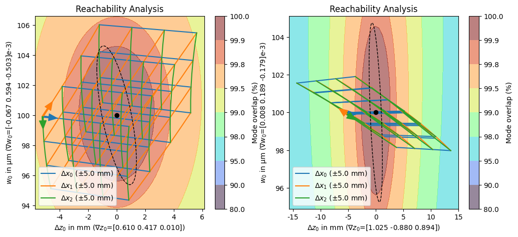
The reachability plot shows which waist positions and radii can be reached by varying the degrees of freedom in a certain range around the calculated optimum represented by a black dot. Assuming perfect alignment, the dashed ellipse represents the confidence region of the waist position and radius, propagated from the fit uncertainty. In another sense, we can also interpret this region as the deviation in waist position and radius that we will likely need to compensate for because of differences in the input beam to our fitted input beam parameters.
The resulting focus and waist positions are evaluated on a grid spanned by all combinations of displacements in the individual degrees of freedom. The points are then connected by colored lines that indicate the degree of freedom that changed between the two points. The direction that corresponds to a positive change in the coordinate is indicated by an arrow starting at the negative most point of all degrees of freedom.
In addition to differentiating waist position from radius, the axis labels also indicate the sensitivity or gradient of the waist position/radius with respect to changes in the degrees of freedom at the optimum.
Finally, the background is a contour plot of the mode overlap for the different final beam positions and radii.
With all this information, we can infer many characteristics of the solution like:
the adjustments in waist position and radius that achieve with reasonable adjustments of the degrees of freedom,
and how these adjustments affect the mode overlap,
this also tells us how (in)sensitive the final beam is to the individual degrees of freedom,
which degree of freedom affects the final beam’s waist position and radius in which way or ratio,
if the actions of the different degrees are sufficiently independent to each other, i.e., orthogonal,
how likely we are to be able to compensate for mode mismatch due to deviations from the fitted input beam parameters.
Comparing the two solutions, we can see that in the least coupled solution (left), the three degrees of freedom are all fairly independent of each other with \(x_0\) (blue) and \(x_2\) (green) almost orthogonal to each other. We can also see, that we will most likely be able to compensate for our fit uncertainties by performing reasonable adjustments to the lens positions that are likely within the range of a translation stage. The strongly coupled (right) solution is pretty much the opposite of this, \(x_1\) (orange) and \(x_2\) (green) are almost perfectly aligned while \(x_0\) (blue) only makes a small angle with them. The result of these couplings is that we require very large and combined movements to achieve a significant correction in the waist radius causing us likely be unable to compensate for the fit uncertainties.
Sensitivity Plot#
As the name would imply, we can create a sensitivity plot using the plot_sensitivity() member function of the respective solution.
[11]:
fig, (axl, axr) = plt.subplots(1, 2, figsize=(12, 5))
solutions_by_coupling[0].plot_sensitivity(ax=axl)
solutions_by_coupling[-1].plot_sensitivity(ax=axr);
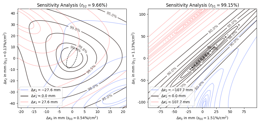
The sensitivity plot, as the name implies, shows how sensitive the mode overlap is to changes in the degrees of freedom or combinations thereof. The plot is a contour plot of the mode overlap as a function of displacements in the two least coupled degrees of freedom. If there are more than two degrees of freedom, the most sensitive remaining degree of freedom is varied in both directions and the resulting contour plots are visualized using different colors. If there are only two degrees of freedom the counter plot is plotted as a contour fill with the same color map as the reachability plot (see next subsection for an example of this). For three or more degrees of freedom only labeled contour lines are drawn to keep the plot readable.
In addition to indicating the respective degrees of freedom, the axis labels also indicate the sensitivity of the respective degree of freedom and the title shows the coupling between the two primary degrees of freedom. And as with the reachability plot, the black dashed ellipse indicates the confidence region propagated from the fit uncertainty. In this case it should be interpreted as the corrections that might be necessary due to deviations from the fitted input beam parameters.
The range for the displacements is automatically chosen so that the 98% mode overlap contour is contained within the plot area. The computation is based on a heuristic so it is not guaranteed that the contour line is always fully visible.
Since mode matching only requires two degrees of freedom, solutions with more than two degrees of freedom are underdetermined. In the mathematical sense, this means that the sensitivity matrix is no longer positive definite, instead it has one zero (or close to zero) eigenvalue per extra degree of freedom. Practically this means, that deviations in one lens can be fully compensated by adjustments in the other lenses without any loss in overlap. This is why the different slices of the auxiliary degree of freedom have mostly the same contour lines. The range of the auxiliary degree of freedom is determined so that the minima within the slices are just within the plotting area. This is also determined heuristically, so the minima are not always guaranteed to be visible.
Comparing the two sensitivity plots, we can see that the inner contour lines of the least coupled (left) solution are fairly circular while the contour lines of the strongly coupled (right) solution are extremely elliptical with non axis aligned major axis. This comparison is also reflected in the coupling values shown in the titles of the plots. This is in some sense the dual representation of the reachability plot, to go from the reachability plot, we distort the plot so that the two primary degrees of freedom are orthogonal and axis aligned. If they already were close to orthogonal the transformation is mostly rotating and scaling. However, if basis vectors were almost pointing in the same direction, the distortion needed to get them orthogonal is much larger which leads to these strongly elliptical contour lines.
As we get farther away from the optimum, the quadratic approximation that a lot of the analysis is based becomes less accurate, and we can see the contour lines distort from their elliptical shape to much more complex forms.
Another important aspect that is somewhat hidden by the automatic range selection is the sensitivity values shown in the axis labels. Due to the strong coupling, the sensitivities of the respective degrees of freedom is three to ten times larger in the strongly coupled solution compared to the least coupled solution.
Conclusion#
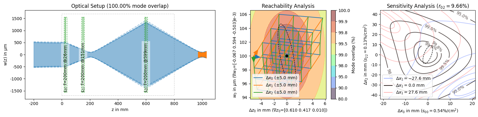
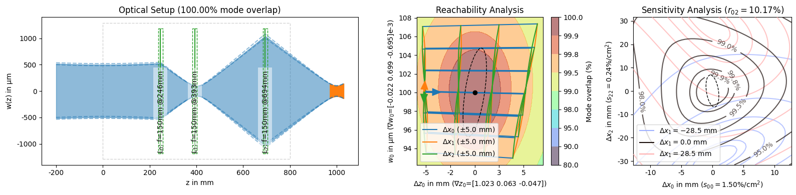
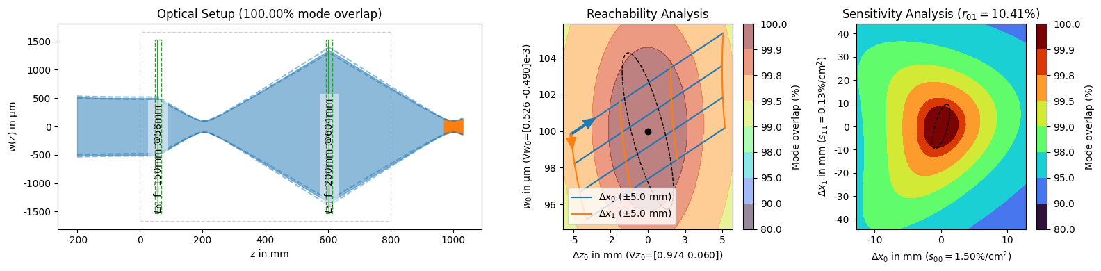
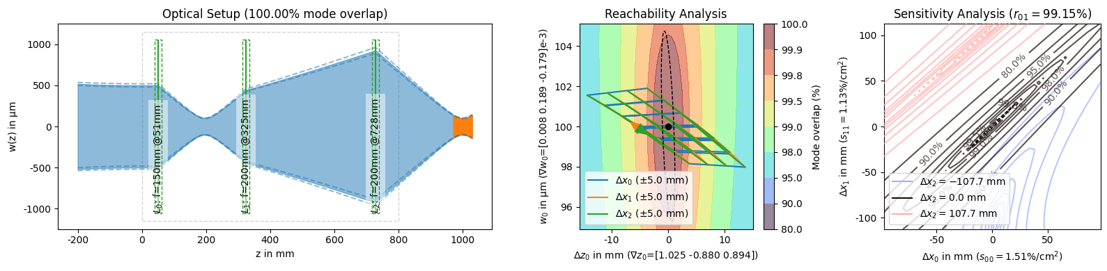
While it is possible to create the reachability and analysis plots by themselves, you will usually invoke them using the plot_all() function which also shows an overview of the mode matching setup in addition to the two analysis plots.
[12]:
solutions_by_coupling[0].plot_all();
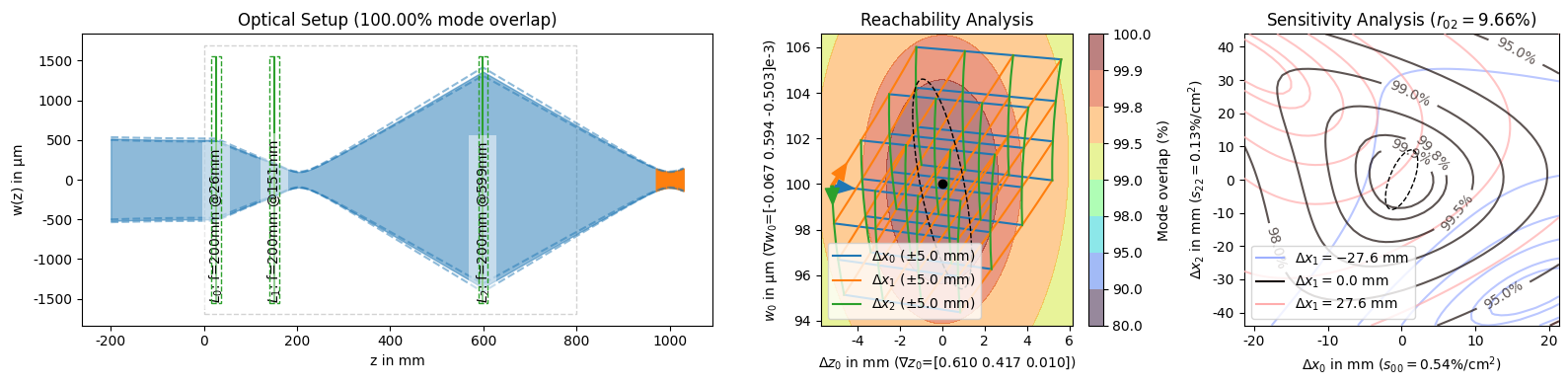
This function is also responsible for creating the PNG representation for solution objects that is shown when a :class:~corset.solver.ModeMatchingSolution is the last expression of a cell or when it is explicitly passed to the :func:~IPython.display.display function. We can use this to easily get an overview of multiple solutions to compare them at a glance.
[13]:
display(*solutions_by_coupling[:3]) # unpack the slice into the display arguments
display(solutions_by_coupling[-1])