Fixed Optics

Beam Corset supports working around existing optics, both in setup characterization and during mode matching.

Characterization with Fixed Optics

When characterizing an existing setup, it may not always be possible or desirable to remove all optics to take beam profile measurements. For these situations, Beam Corset also allows beam characterization with existing optics in place. Instead of using Beam.fit(), we use OpticalSetup.fit() which works similarly but also takes in a list of tuples of lens positions and optical elements.

from corset import Beam, OpticalSetup, ThinLens
import numpy as np
import matplotlib.pyplot as plt

np.random.seed(42)

# generate reference setup
lens = ThinLens(200e-3)
ref_beam = Beam.from_gauss(focus=0.1, waist=300e-6, wavelength=1064e-9)
ref_setup = OpticalSetup(ref_beam, [(0.2, lens)])

# generate noisy measurements
meas_positions = np.linspace(0.0, 0.4, 10)
meas_radii = ref_setup.radius(meas_positions) + np.random.normal(0, 10e-6, size=len(meas_positions))

fit_setup = OpticalSetup.fit(meas_positions, meas_radii, ref_beam.wavelength, [(0.2, lens)])
fit_beam = fit_setup.initial_beam

print(f"Reference beam: focus = {ref_beam.focus*1e3:.1f}mm, waist = {ref_beam.waist*1e6:.1f}μm")
print(
    f"Fitted beam: focus = ({fit_beam.focus*1e3:.1f}±{fit_beam.gauss_cov[0,0]**0.5*1.96e3:.1f})mm",
    f"waist = ({fit_beam.waist*1e6:.1f}±{fit_beam.gauss_cov[1,1]**0.5*1.96e6:.1f})μm",
)

plt.plot(meas_positions, meas_radii, "o", label="Measurements")
plt.legend()
fit_setup.plot(show_legend=True);

Reference beam: focus = 100.0mm, waist = 300.0μm
Fitted beam: focus = (91.5±16.7)mm waist = (303.7±6.7)μm

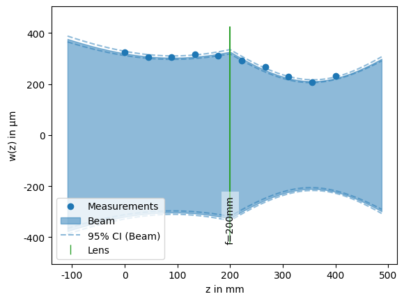
One problem with this approach is that it relies on knowing the exact position of the existing lens. If the assumed lens position deviates from the true lens position, the fitted beam parameters will likely be off as well, leading to unusable mode matching results down the line.

To prevent this, we can include the lens position as a free parameter in the fit. To do this, we replace the lens position with a tuple of the estimated position and a maximum deviation from that position. Note that since we are not fitting an additional parameter, we will need to provide more measurements to achieve the same level statistical confidence.

fit_setup_lens = OpticalSetup.fit(meas_positions, meas_radii, ref_beam.wavelength, [((0.2, 0.01), lens)])
fit_beam_lens = fit_setup_lens.initial_beam
print(f"Reference beam: focus = {ref_beam.focus*1e3:.1f}mm, waist = {ref_beam.waist*1e6:.1f}μm")
print(
    f"Fitted beam: focus = ({fit_beam_lens.focus*1e3:.1f}±{fit_beam_lens.gauss_cov[0,0]**0.5*1.96e3:.1f})mm",
    f"waist = ({fit_beam_lens.waist*1e6:.1f}±{fit_beam_lens.gauss_cov[1,1]**0.5*1.96e6:.1f})μm",
)
print(f"Fitted lens position = {fit_setup_lens.elements[0][0]*1e3:.1f}mm")

Reference beam: focus = 100.0mm, waist = 300.0μm
Fitted beam: focus = (92.7±28.5)mm waist = (303.6±7.6)μm
Fitted lens position = 200.6mm

We can see that the uncertainty increases when fitting with the lens, because the same amount of measurement information now needs to constrain an additional parameter and we can effectively do less averaging.

Mode Matching with Fixed Optics

We can also account for fixed optics during mode matching. This may be needed when a cavity’s in-coupler has curved surfaces. This works the same as normal mode matching, except that we pass an optical setup to the mode_match() call instead in place the initial beam. The fixed optics do not participate in the optimization, but are still respected when propagating the beam through the setup. Since they are assumed to be immovable, they are also excluded from the analysis.

from corset import ShiftingRange, mode_match

initial_beam = Beam.from_gauss(focus=0.0, waist=500e-6, wavelength=1064e-9)
initial_setup = OpticalSetup(initial_beam, [(0.95, ThinLens(100e-3))])
desired_beam = Beam.from_gauss(focus=1.0, waist=50e-6, wavelength=initial_beam.wavelength)

solutions = mode_match(
    initial_setup, # pass an optical setup that includes the fixed optic(s)
    desired_beam,
    [ShiftingRange(0.0, 0.8)],
    [ThinLens(f) for f in [100e-3, 150e-3]],
    max_elements=2,
)
solutions[2]

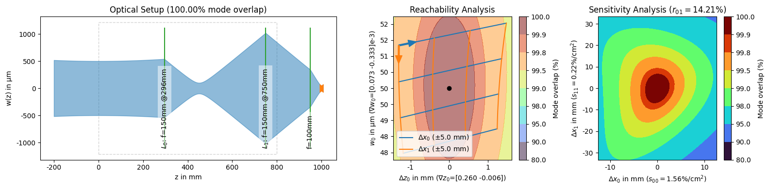
The fixed optics does not get its own \(L_n\) degree of freedom and is simply displayed as is.