Beam Constraints

In some mode matching scenarios, it is not only critical, that the final beam matches the desired mode, the beam must also fit through various other optics along the way. To account for this during mode matching, the relevant optics can be modelled as additional constraints on the beam radius at various positions. The solver will then only consider solutions that satisfy these constraints.

Note

Due to the more thorough evaluation of the beam shape, combined with the additional complexity of constrained optimization, solving with constraints can be significantly slower.

Note

While most mode matching problems only have a single global optimum, some problems, especially constrained mode matching problems may have local imperfect optima. Since the solver uses a local optimization method, it may not find a mode matching for a given lens population subject to constraints. To reduce the chances of missing a solution, you can direct the solver to try additional pseudo random (seeded with random_seed) initial position in addition to the deterministic initial guess. This can be specified with the random_initial_positions parameter in the mode_match() function. While approximately (specified by equal_setup_tol) equal solutions will be deduplicated, this may still lead similar solutions. To prevent this you can limit the amount of solutions per candidate with the solutions_per_candidate parameter.

Apertures

The simplest type of constraint is an aperture constraint. It can be used to model optics that are thin compared to the Rayleigh range of the beam such that the beam radius can be approximated as constant over the thickness of the optic. These constraints are modelled using the Aperture class.

An aperture is specified by its position along the optical axis and its radius. Additionally, power fraction can be specified to set a lower limit on the fraction of power that must pass through the aperture. The default value for the power fraction is $1-e^{-2} \approx 0.865$, with this, the specified radius determines the maximum $1/e$ field radius at that point.

from corset import Aperture

basic_aperture = Aperture(position=0, radius=500e-6)
aperture_with_power = Aperture(position=0, radius=500e-6, power=0.99)

During the optimization process, all apertures are converted to equivalent \(1/e\) radius constraints. If the power fraction is larger than \(1-e^{-2}\), the equivalent \(1/e\) radius is simply decreased to ensure that the specified power fraction passes through the specified aperture radius.

print(basic_aperture.radius_constraints) # [(position, radius)]
print(aperture_with_power.radius_constraints) # reduced 1/e radius

[(0, np.float64(0.0005))]
[(0, np.float64(0.0003295051144911304))]

Passages

Elements that have a thickness, or in these cases a length, over which the beam radius may significantly change, can be modelled using the Passage class. A passage is specified by its starting (left) and ending (right) position along the optical axis, as well as its radius and an optional power fraction. Alternatively the passage position can also be specified using its center position and width.

from corset import Passage

simple_passage = Passage(left=0, right=0.1, radius=500e-6)
centered_passage = Passage.centered(center=0.05, width=0.1, radius=500e-6)

Internally, passages are represented as two apertures at the start and end respectively. For this to work, no optics must be placed within the passage, this is enforced by the solver. This also means that the power fraction is only an approximation, that assumes, that only one of the two apertures causes significant clipping of the beam. This should be the case in most situations, but in the unlikely case, that the beam radius is similar at both ends, the actual power loss might be slightly higher than specified.

simple_passage.radius_constraints  # [(left, radius), (right, radius)]

[(0, np.float64(0.0005)), (0.1, np.float64(0.0005))]

Focuses

In some cases, it may be important to have a focus at a certain position without requiring a specific waist radius. This may be because a flat wavefront curvature is required. Instead of performing a separate mode matching with a haphazardly chosen waist radius, thereby unnecessarily constraining the problem with a specific waist radius that we do not actually care about, we can use a Focus constraint to specify the focus position without constraining the waist radius. As implied, the only parameter to this constraint is the desired position of the focus.

from corset import Focus

Focus(position=0.1)

Focus(position=0.1)

Note

While the Aperture and Passage constraints typically only determine whether a certain lens population candidate can mode match while satisfying the constraints, otherwise leaving the degrees of freedom mostly free, Focus constraints are equality constraints and therefore also always “consume” a degree of freedom. This when using these constraints, we require an additional lens for every one of the so that we are still left with two degrees of freedom to achieve perfect mode overlap.

Tip

Combine a Focus with an Aperture directly on top of it to limit the radius of the arbitrary beam waist radius.

Example

Let’s look at a minimal example to demonstrate the usage of apertures, passages, and focus constraints. Since the initial and final beam are fixed and will be the same for every potential solution, beam constraints only make sense between shifting ranges where the beam shape can actually differ. We will not use power fractions to make it easier to see that the constraints are actually satisfied.

from IPython.display import display
from corset import Beam, ShiftingRange, ThinLens, mode_match

initial_beam = Beam.from_gauss(focus=0, waist=200e-6, wavelength=1064e-9)
desired_beam = Beam.from_gauss(focus=1.2, waist=300e-6, wavelength=initial_beam.wavelength)
ranges = [ShiftingRange(0, 0.25), ShiftingRange(0.5, 0.75), ShiftingRange(0.85, 1.1)]
lenses = [ThinLens(f) for f in [0.1, 0.15, 0.2]]
constraints = [
    Passage(left=0.3, right=0.4, radius=400e-6),
    Aperture(position=0.45, radius=300e-6),
    Focus(position=0.8),
    # optionally constraint the maximum waist radius at the
    # focus constraint to filter out the second solution
    # Aperture(position=0.8, radius=200e-6),
]

solutions = mode_match(initial_beam, desired_beam, ranges, lenses, max_elements=3, constraints=constraints)
solutions

	overlap	num_elements	elements	positions	min_sensitivity_axis	min_sensitivity	max_sensitivity_axis	max_sensitivity	min_cross_sens_pair	min_cross_sens	min_cross_sens_direction	min_coupling_pair	min_coupling	sensitivities	couplings	const_space	grad_focus	grad_waist	sensitivity_unit	solution
0	1.0	3	[f=150mm, f=100mm, f=100mm]	[0.18073917330283817, 0.6720856549309916, 0.91...	0	0.232926	2	2.066657	(0, 1)	0.166437	[0.9951895974947432, -0.09796767343491904]	(0, 1)	0.249709	[[0.23292608513848276, 0.16643654886593734, -0...	[[0.9999999999999999, 0.2497091492725869, -0.4...	[[-0.45282447039968715, -0.6148791737382567, -...	[-3.6260457907062937, -2.3085403504133977, 4.7...	[5.75372229706104e-05, 0.005712499050498045, -...	SensitivityUnit.PERCENT_PER_CM2	ModeMatchingSolution(candidate=ModeMatchingCan...
1	1.0	3	[f=150mm, f=150mm, f=200mm]	[0.2163513489629172, 0.6233330901560286, 1.000...	2	0.135058	0	0.224991	(0, 2)	0.105657	[0.5515440196698329, -0.8341457872377244]	(0, 2)	0.606116	[[0.22499098537039453, -0.16490995005347678, 0...	[[0.9999999999999999, -0.7380207309078957, 0.6...	[[0.1487768740748541, 0.6693449153182385, 0.72...	[2.159930907055802, -3.4839540926290447, 2.762...	[-0.0016010471773264985, 0.0003564465000770287...	SensitivityUnit.PERCENT_PER_CM2	ModeMatchingSolution(candidate=ModeMatchingCan...

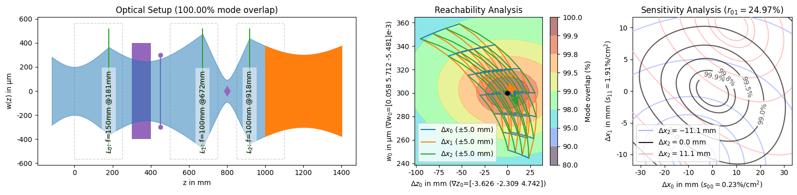
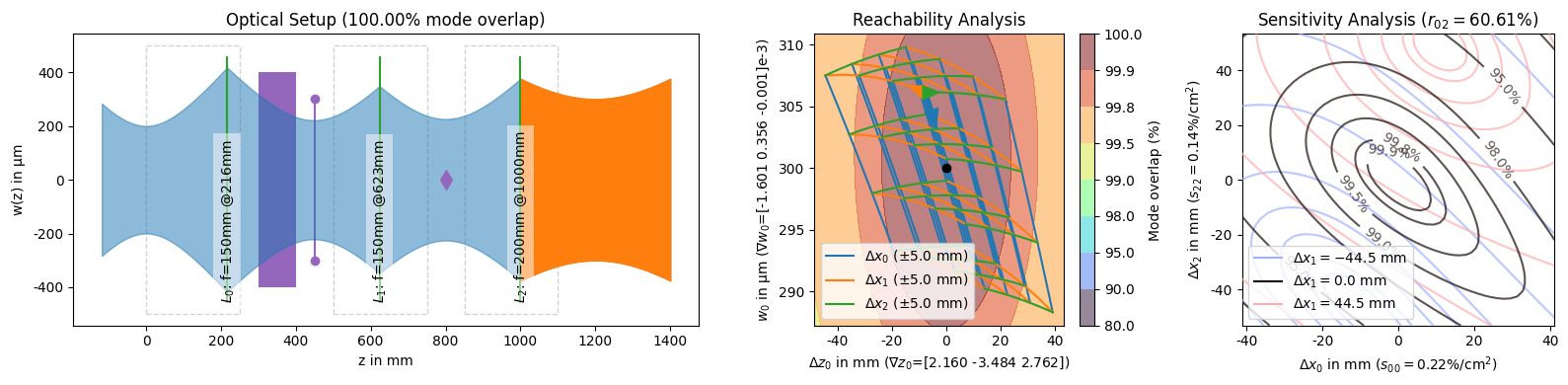
The constraints are visualized in the setup plot as rectangles and vertical handles for the passages and apertures respectively. The size shown is always the specified radius, not the equivalent \(1/e\) radius, so depending on the specified power fraction the beam may never be able to reach the edge or may even surpass it for very low power fractions. Focus constraint are visualized with a diamond at the desired focus position.

display(*solutions)

To verify that the constraints were not satisfied by pure luck, we can rerun the search without constraints, and we will see that we will get additional solutions that did not meet the constraints.

unconstrained_solutions = mode_match(initial_beam, desired_beam, ranges, lenses, max_elements=3)
print(f"Found {len(unconstrained_solutions)} solutions") # many more solutions than before

Found 51 solutions